A cluttered Excel sheet can be a nightmare—extra spaces, inconsistent formatting, random text everywhere. But with the right functions, you can clean it up in seconds and make your data actually usable.
5
TRIM
Stray spaces on your spreadsheet can make two identical-looking entries different, mess with data validation, and even throw off your formulas. Thankfully, the TRIM function solves all that by removing all extra spaces from your texts (except single spaces between words). This function is great for tidying up names, addresses, etc., especially in the sheets you import from other sources.
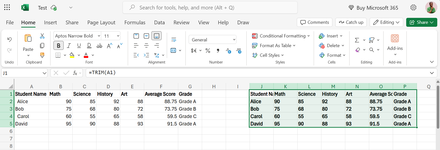
Let’s say cell A1 contains Alice, with extra spaces everywhere. Using the TRIM function will return Alice with no spaces.
Instead of referencing one cell and extending the formula, you can also reference all your data in one go. For instance, I can use the following formula to clean all my stray spaces.
=TRIM(A1:G5)
TRIM is often your first line of defense in data cleanup. Many other text functions work better when you’ve already trimmed your data, so don’t skip this step.
4
IFERROR
I instantly feel like an amateur whenever I have DIV/0, N/A, VALUE!, and all other fancy Excel errors littered across my spreadsheets. Maybe I don’t feel that way all the time, but just the sight of them makes me (and my colleagues) so anxious over something that could very well be a little issue.
IFERROR displays something more presentable and less anxiety-inducing. It works with Office 2019 and Microsoft 365 subscriptions, so it’s widely accessible. This function evaluates a formula and returns a specified value if the formula results in an error.
For instance, instead of using a formula that returns #NAME? when no match is found, such as the one below:
=VLOOKUP(A1,Table1,2,FALSE)
You can use the following formula to return a custom message instead:
=IFERROR(VLOOKUP(A1,Table1,2,FALSE),"Not Found")
Your spreadsheet instantly looks more professional, and your boss stops asking why there are error messages everywhere. Plus, you can return whatever you like—blank cells, a dash, custom messages, or even alternative calculations—if and when errors occur.
3
CLEAN
When you import data from PDFs, websites, and legacy systems or even convert PDF files into Excel spreadsheets, you tend to carry along some invisible characters. Things like line breaks and hidden symbols, which you can’t see, can tag along and break your formulas.
The CLEAN function removes all non-printable characters from your text, leaving behind a more predictable and formula-friendly version.
You can also pair CLEAN with the TRIM function. Many Excel pros use this as their go-to combo for imported data:
=TRIM(CLEAN(text))
CLEAN removes the first 32 non-printable characters in the 7-bit ASCII code (values 0 through 31), which works for Windows-based files. If your data comes from macOS or web sources, you might need additional tools to clean out Unicode nuisances.
2
TEXTSPLIT
Sometimes, all your data ends up crammed into a single cell, separated by commas, semicolons, periods, or line breaks. Having to then extract your data into appropriate rows and columns manually is a pain.
TEXTSPLIT, available in Excel 365 and Excel 2021, works the same as the Text-to-Columns wizard, but in formula form, and it’s great if you’re dealing with concatenated data. This function can split text across columns or down rows using delimiters you specify.
If cell A1 contains Ada,Uche,ada.uche@email.com, then using the formula below can split the text into three separate columns: Ada, Uche, and ada.uche@email.com.
=TEXTSPLIT(A1,",")
You can even split by row or column, and handle multiple delimiters. For instance, if cell A2 contains Apple,Banana;Cherry, then use the formula below:
=TEXTSPLIT(A1, {",", ";"})
This will split the text into Apple, Banana, and Cherry.
By default, TEXTSPLIT will fill these values across columns. If you wanted them to split into separate rows instead, set the fourth argument, which is FALSE or omitted by default, to TRUE:
=TEXTSPLIT(A2, ",",";", , TRUE)
This would result in Apple in cell I1, Banana in J1, Cherry in I2, and Dates in J2.
Notice that you’d be using one delimiter (like a semicolon) to split words into columns, and another (like a period) to indicate where a new row should begin.
As a result, this function can get quite complex. It often requires careful planning of your delimiters and potentially combining TEXTSPLIT with other functions to achieve your desired layout. But for extraction, TEXTSPLIT works great.
1
TEXTJOIN
After splitting, you may want to stitch the pieces back. TEXTJOIN helps you merge multiple text strings with a delimiter of your choice and even lets you skip blanks.
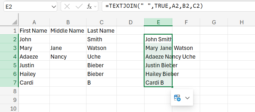
Let’s say you have first names in column A, middle names in column B (some cells are empty), and last names in column C. You can use the following formula to create full names without extra spaces from empty middle name cells.
=TEXTJOIN(" ",TRUE,A1,B1,C1)
You’ll get full names like Cardi B or Mary Jane Watson after applying the formula.
The TRUE argument tells Excel to ignore empty cells, so you don’t get awkward gaps or dangling commas.
Messy spreadsheets are chaotic until you sort them out. But with the right Excel functions, you don’t need hours of manual fixing. So, the next time you open a spreadsheet that makes your eyes twitch, you’ll know exactly what to do.


