Whether you’re applying for a role that requires Excel expertise, want to add more strings to your data analysis bow, or simply want to do more with your data in Microsoft’s spreadsheet program, add these five Excel skills to your toolkit to unlock the next level.
1
Excel Tables: Organize Your Data
Raw Microsoft Excel data can be in a regular range or a table. A regular range is a collection of cells that are not structurally connected, while a table is an object containing column headers, fields (columns), records (rows), and other features.
When formatted as an Excel table, your figures instantly become more readable, you can easily filter and sort your data, and you can reference specific column headers in formulas to aid accuracy and save time.
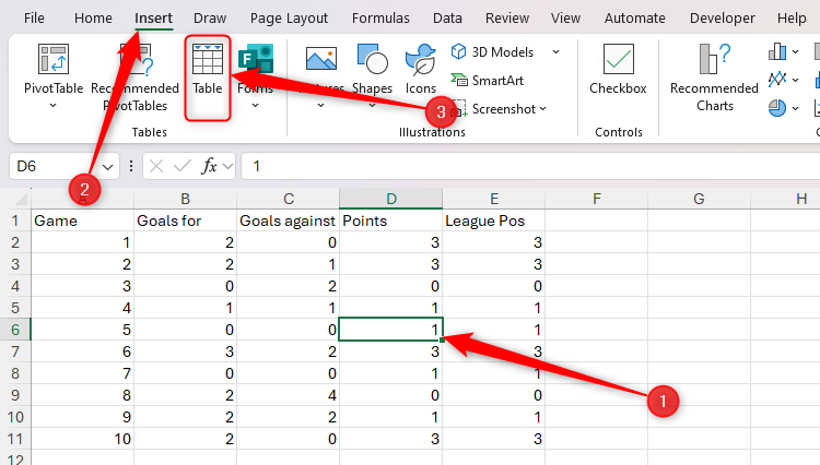
To convert your data into a table, select all the cells in the range (including the header row). Alternatively, if your range is contiguous (in other words, all the cells are next to each other with no blank columns or rows), you can select a single cell in the data instead. Then, in the Insert tab on the ribbon, click “Table.” If you prefer using keyboard shortcuts in Microsoft Excel, press Ctrl+T.
Make sure you have column headers along the top row before you convert your range. Taking this step makes dealing with and using the data more straightforward later on.
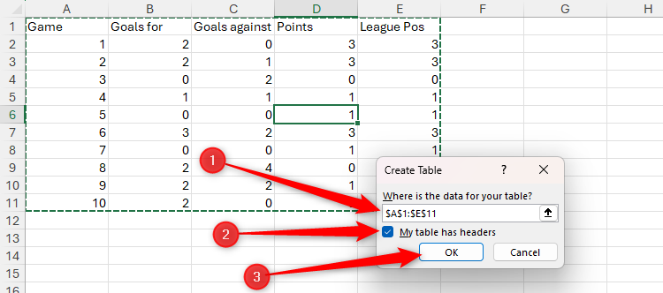
Next, in the Create Table dialog box, verify that the whole range is selected, check “My Table Has Headers,” and click “OK.”
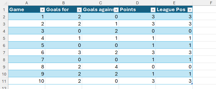
And there you have it! A nicely formatted table with filter buttons added to your column headers.
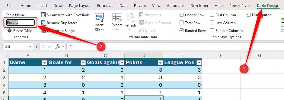
By default, tables are named Table1, Table2, Table 3, and so on, but if you rename a table in the Properties group of the Table design tab, this makes your spreadsheet more navigable, helps people using screen readers, and makes formula creation and understanding easier if they reference a column in the table.
Table names must start with a letter, underscore, or backslash, with the other characters being letters, numbers, periods, or underscores. They must also be unique, can’t contain a space, and mustn’t have the same name as a cell reference, like A1.
In the same tab, you can change the table design or choose which elements your table contains.
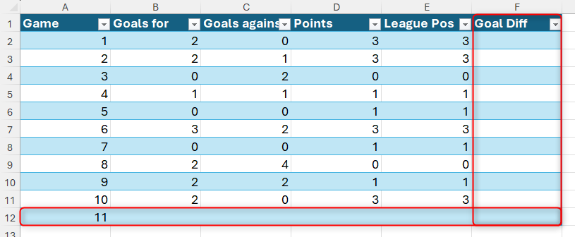
One of the benefits of formatted Excel tables is that adding columns and rows is really simple. Here, as soon as I typed a column header into cell F1 and a game number into cell A12, Excel expanded the table to capture the extra data.
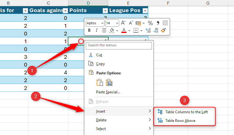
On the other hand, to insert a column or row in the center of your table, right-click a cell, hover over “Insert,” and choose the appropriate option.
Here’s a summary of the pros and cons of using tables in Excel:
|
Pros of Excel Tables |
Cons of Excel Tables |
|---|---|
|
Formulas in tables automatically extend to new rows. |
They’re incompatible with dynamic array formulas. |
|
Tables make sorting and filtering easy. |
Having too many tables in a workbook can hamper its performance. |
|
You can quickly and easily format a table for enhanced visualization. |
Tables can’t accommodate non-standard data structures (though this is probably a pro rather than a con, as they force you to structure your data correctly). |
|
Tables have handy optional features, like a total row and banding. |
|
|
Data formatted as a table is more compatible with other Excel tools, like Power Query and charts. |
2
Power Query: Import and Shape Your Data
When I learned about Power Query in Excel, it completely changed how I deal with my data. This tool works by connecting to a single or multiple data sources, from which you can extract the necessary information. Then, you can transform and clean your extracted data to meet your needs, and load the result onto a worksheet.
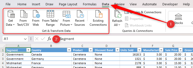
To begin, head to the “Data” tab on the ribbon, and tell Excel where the data source is located, either from one of the options immediately visible or through the Get Data drop-down menu.
Specifically, you can use Power Query to import a single dataset like an Excel workbook, a table from a website, or a database. Alternatively, you can import multiple datasets from worksheets in an Excel file or more than one Excel workbook.
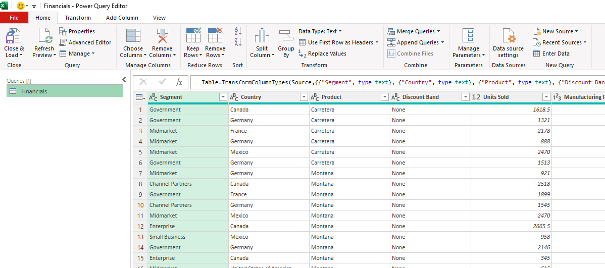
Once you’ve identified the data source, you’re taken to the Power Query Editor, where you’ll do most of your data transformations.
For example, in the Home tab, you can add new sources, manage the parameters, split columns, append queries, and perform a whole host of other common actions. In the Transform tab, you can make changes to existing data, like splitting columns, transposing the data structure, replacing values, extracting text, and much more.
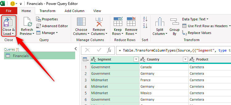
After you’ve finished making the relevant data transformations, click “Close And Load” in the top-left corner of the Power Query Editor window. Specifically, clicking the top half of the split button automatically loads the data onto a new worksheet, while clicking the bottom half gives you more loading options.
To ensure that the resultant table always reflects any changes in the data source, routinely click “Refresh” in the Table Design tab on the ribbon.
Before you go ahead and use this tool, take a moment to review its strengths and drawbacks:
|
Pros of Power Query |
Cons of Power Query |
|---|---|
|
Power Query is user-friendly with an intuitive interface. |
As with many advanced tools in Excel, overusing Power Query can be resource-intensive. Apply filters early and reduce the number of steps to limit its impact on performance. |
|
It’s a real time-saver—without this tool, transforming, cleaning, and combining data would be cumbersome and likely to lead to errors. |
To make the most of Power Query’s capabilities, you’ll need to master M language, Power Query’s programming language. |
|
Since Power Query extracts data from the source, the original data remains intact. |
|
|
The tool can work flexibly with data of various sizes from sources outside Excel. |
3
Data Validation: Restrict Data Entries
Whether you use Excel at home or in the workplace, data validation is something that all power users know like the back of their hand. What’s more, beyond fundamental data entry restriction, the data validation tool can be used to power dynamic charts and create cascading drop-down lists.
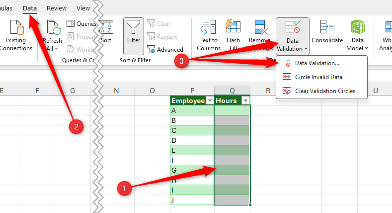
To get started, select the relevant cell or cells, and in the Data tab on the ribbon, click “Data Validation.” If you see a drop-down menu, click “Data Validation” again.
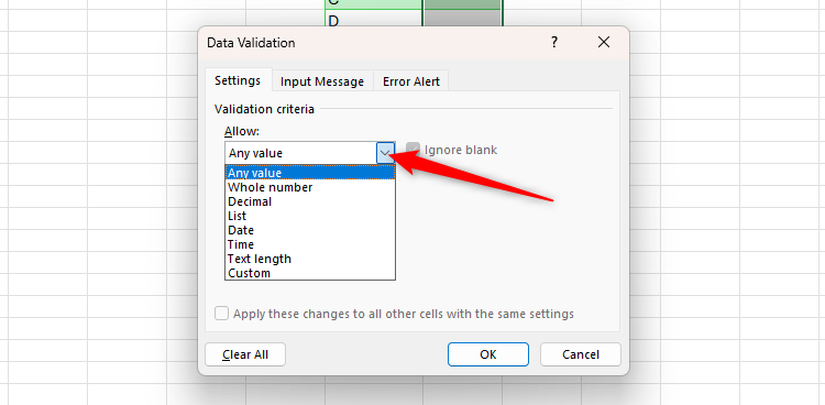
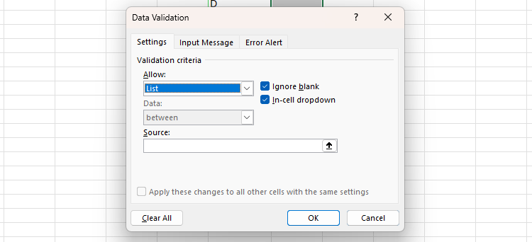
Then, in the Allow field, select a data type.
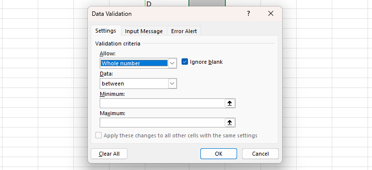
For example, clicking “Whole Number” brings up additional fields where you can specify the parameters.
On the other hand, if you choose “List,” you can reference cells or a named range to add a drop-down list to the selected cells.
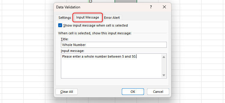
As well as limiting what can be entered into a cell, Data Validation also lets you add an input message that appears when a cell is selected. Simply head to the “Input Message” tab, and fill in the fields.
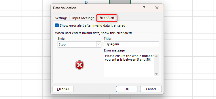
Finally, you can define the alert that appears when the wrong data type is entered in the Error Alert tab.
Here’s a summary of the benefits of using data validation in Excel, as well as some caveats you should be aware of:
|
Pros of Data Validation |
Cons of Data Validation |
|---|---|
|
Data validation improves accuracy, consistency, and efficiency. |
Data validation rules aren’t foolproof—cells can be overridden, and conditions can be altered. |
|
The tool can help others understand your workbook if you plan to share it. |
You can’t use table column headers as the source of a list. However, you can get around this by creating a named range. |
|
Creating data validation rules, messages, and alerts is straightforward. |
|
|
When used to its maximum potential, data validation can be essential for decision-making and analysis. |
|
|
As well as restricting data inputs in certain cells, data validation rules are essential in dynamic worksheets, like dashboards and forms, as they can be used to drive live charts and dependent drop-down lists. |
4
PivotTables: Summarize and Analyze Large Datasets
In their simplest form, PivotTables condense and reorganize large datasets for instant analysis in Excel. After all, worksheets containing hundreds of rows and columns can be overwhelming and difficult to read.
However, once you take some time to play around with them, you’ll realize that PivotTables are an incredibly powerful tool that can do more than you initially thought.
To turn your Excel table into a PivotTable, select any cell in the range, and in the Insert tab, click the top half of the split “PivotTable” button.
To create a PivotTable from a source outside Excel, click the bottom half of the “PivotTable” icon, and select “From External Data Source.”
Then, in the dialog box, confirm that the correct range or table name is selected, and decide whether you want the PivotTable to be added to the active worksheet or a new one.
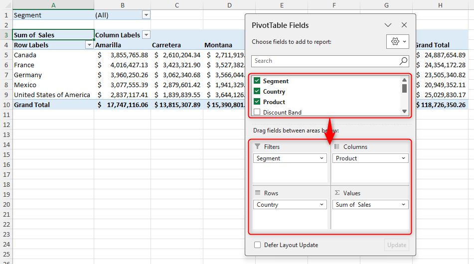
Now, in the PivotTable Fields pane, click and drag the relevant fields into one of the following areas:
- Rows: These are the fields that sit in the first column of the PivotTable.
- Columns: These are the fields that appear as column labels along the top row of the PivotTable.
- Values: The fields placed in this area are aggregated in the rightmost column of the PivotTable. You can change how the data is aggregated by clicking the down arrow next to the field name once you’ve added it to the Values area.
- Filters: You can filter the whole PivotTable based on a field you add to the Filters area.
To remove a field from a PivotTable area, click and drag it away from the PivotTable Fields pane.
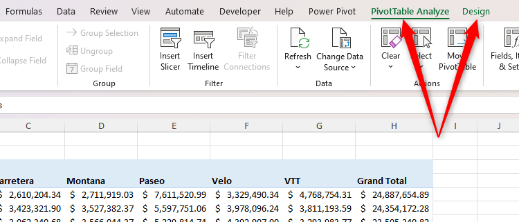
Once you’ve selected the fields you want to be on display in the PivotTable, you can change its layout in the Design tab, or access advanced tools, such as timelines and slicers, in the “PivotTable Analyze” tab.
With your PivotTable set up, you can quickly perform advanced tasks that would take much longer if you did them manually, like showing values as a percentage of the total, filtering the top values, and even creating individual reports based on a filter.
Here are the pros and cons of using PivotTables in Excel:
|
Pros of PivotTables |
Cons of PivotTables |
|---|---|
|
PivotTables let you summarize, aggregate, filter, and sort large datasets in seconds. |
If you’re using an older version of Excel, you need to refresh PivotTables manually if the source data changes. |
|
You can quickly change the rows, columns, filters, and totals to visualize your data in the most appropriate way. |
PivotTables based on large datasets can consume lots of memory, slowing your computer significantly. |
|
PivotTables come with advanced filtering options, like slicers and timelines, making data analysis even easier. |
|
|
You can use PivotTables to drive PivotCharts that further aid data visualization. |
5
XLOOKUP: Find and Retrieve Data
Finding the right functions to learn if you’re looking to elevate your Excel expertise can be challenging because there are so many. However, if I had to choose one, it would be XLOOKUP.
XLOOKUP searches for a value in a range and returns a corresponding value from another column or row, turning your Excel file into a dynamic workbook with interlinking datasets. Here’s the syntax:
=XLOOKUP(a,b,c,d,e,f)
where
- a (required) is the lookup value,
- b (required) is the lookup array,
- c (required) is the return array,
- d (optional) is the text to return if the lookup value (a) is not found in the lookup array (b),
- e (optional) is the match mode (0 = exact match; -1 = exact match or next smaller item; 1 = exact match or next larger item; 2 = a wildcard match), and
- f (optional) is the search mode (1 = starting at the first item; -1 = starting at the last item; 2 = binary search relying on the array being in ascending order; -2 = binary search relying on the array being in descending order).
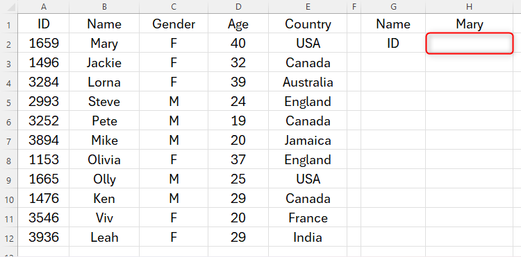
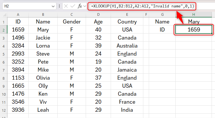
In this example, I want Excel to look up the employee ID based on the name in cell H1, and return the result to cell H2.
To do this, I need to type the following formula:
=XLOOKUP(H1,B2:B12,A2:A12,"Invalid name",0,1)
where
- H1 references the value Excel needs to look up (Mary),
- B2:B12 is the array containing the value I’m looking up,
- A2:A12 is the array containing the value I want to return,
- “Invalid Name“ is what I want Excel to return if the lookup value isn’t anywhere to be found in the lookup array,
- 0 tells Excel that I want an exact match, and
- 1 tells Excel to start from the top.
XLOOKUP is a more powerful and flexible alternative to VLOOKUP, which only works with vertical datasets, and HLOOKUP, which only works with horizontal datasets. What’s more, you can use XLOOKUP to perform two-dimensional lookups, returning a value at the intersection of a specified column and row.
Here’s a summary of the strengths and weaknesses of this useful lookup function:
|
Pros of XLOOKUP |
Cons of XLOOKUP |
|---|---|
|
XLOOKUP is the best way to return a value based on a corresponding match. |
This function is only available in versions of Excel released in 2021 or later. |
|
Unlike other lookup functions, you can enter an if not found argument to deal with errors. |
Other lookup functions (particularly INDEX and MATCH) are considered more flexible when working with non-contiguous columns. |
|
You can use this function to extract data from vertical and horizontal datasets. |
|
|
You can nest XLOOKUP to perform two-way lookups. |
|
|
XLOOKUP doesn’t require the data to be sorted. |
|
|
This function can return more than one value from a single lookup. |
To put your Excel expertise under the microscope, have a go at the How-To Geek Advanced Excel Test!
