Slow lookup formulas can kill productivity when working with large datasets. To cope with that, I’ve tested Excel’s optimal lookup functions and their combinations for building lightning-fast formulas that handle even massive spreadsheets with ease.
4
XLOOKUP Is My Go-To Functions
It’s Much Better Than VLOOKUP
I have used VLOOKUP for a long time, but it has limitations with complex data. XLOOKUP, on the other hand, eliminates most of these problems while offering better performance and flexibility.
When using XLOOKUP, you select the lookup and return columns separately, meaning you can finally look to the left of your lookup column without rearranging your data. That’s one of the reasons why XLOOKUP is better than VLOOKUP.
XLOOKUP has the following syntax:
=XLOOKUP(lookup_value, lookup_array, return_array, [if_not_found], [match_mode], [search_mode])
Let’s break down the parameters:
- lookup_value: What you’re looking for.
- lookup_array: The range or array where you’ll search.
- return_array: Holds the values you want to retrieve.
The optional parameters give you more control:
- [if_not_found]: Lets you specify custom error messages instead of seeing common Excel errors like #N/A and eliminates the need for IFERROR.
- [match_mode]: Offers exact matches, wildcards, or approximate matches.
- [search_mode]: Determines whether Excel searches from first to last or last to first.
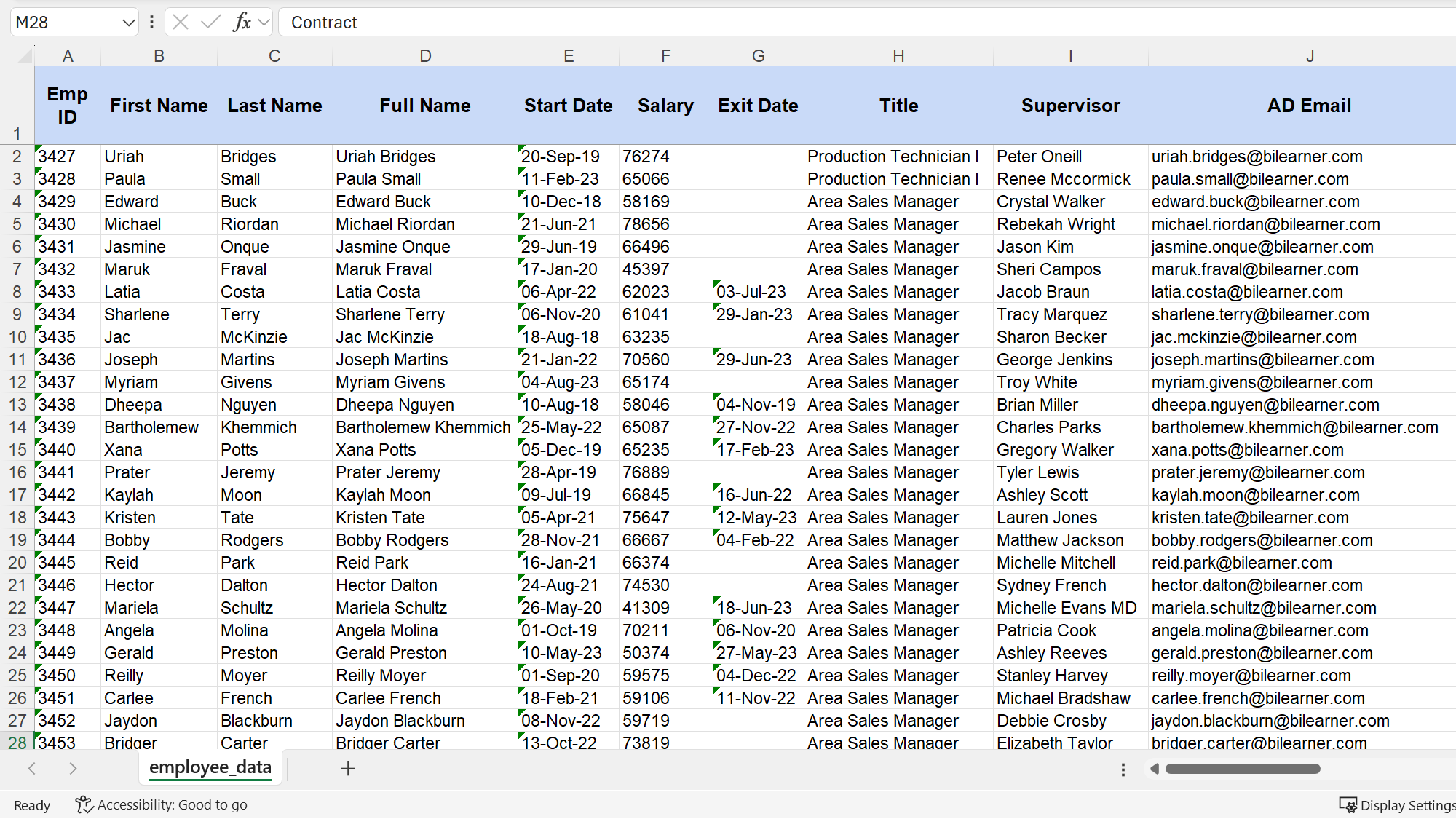
Let’s use an office-related example. If you have an employee’s email address and need to find their full name, you will have to do so by looking to the left. VLOOKUP can’t do this easily because the “Full Name” column is to the left of the “AD Email” column. But it’s doable with XLOOKUP.
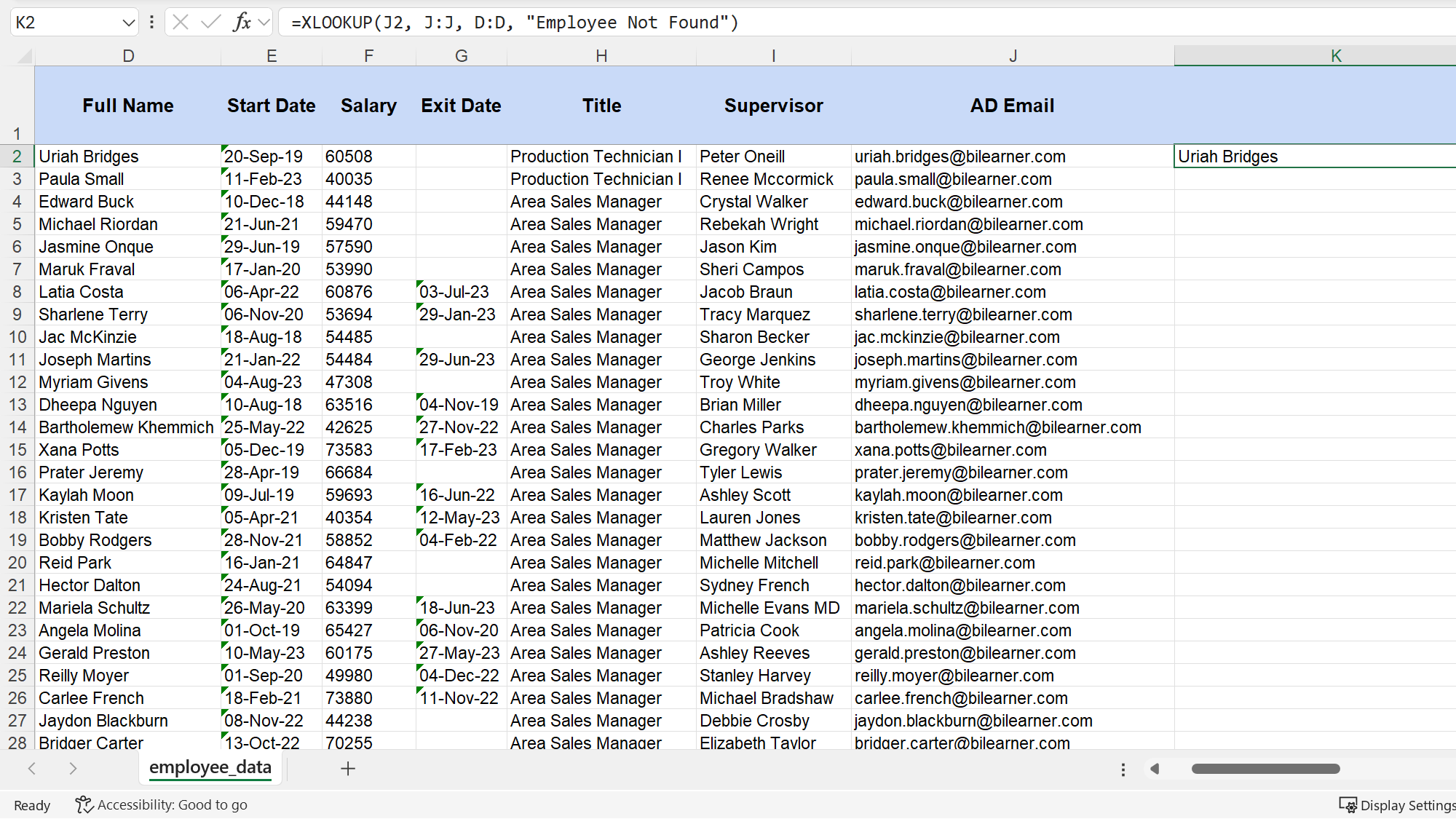
For instance, if you have the email address uriah.bridges@bilearner.com in cell J2, you can use this formula to find the full name:
=XLOOKUP(J2, J:J, D:D, "Employee Not Found")
Here, the formula searches for the email in column J and returns the corresponding name from column D. If the email isn’t found, it cleanly returns “Employee Not Found” instead of a jarring #N/A error. This built-in error handling makes it more robust and user-friendly.
3
I Combine LET and XLOOKUP
Eliminate Repetitive Calculations
Formulas can sometimes become long and complex, especially when you need to perform the same calculation multiple times within a single formula. This not only makes the formula hard to read but also hurts performance, as Excel has to compute the same result repeatedly.
The solution to this is the LET function, which allows you to declare variables directly inside a formula. You calculate something once, give it a name, and then just use that name whenever you need the result. The syntax is simple:
=LET(name1, name_value1, [name2, name_value2], calculation)
- name1: The name for your first calculation (e.g., “rating”).
- name_value1: The calculation itself (e.g., an XLOOKUP formula).
- calculation: The final formula that uses the name you just defined.
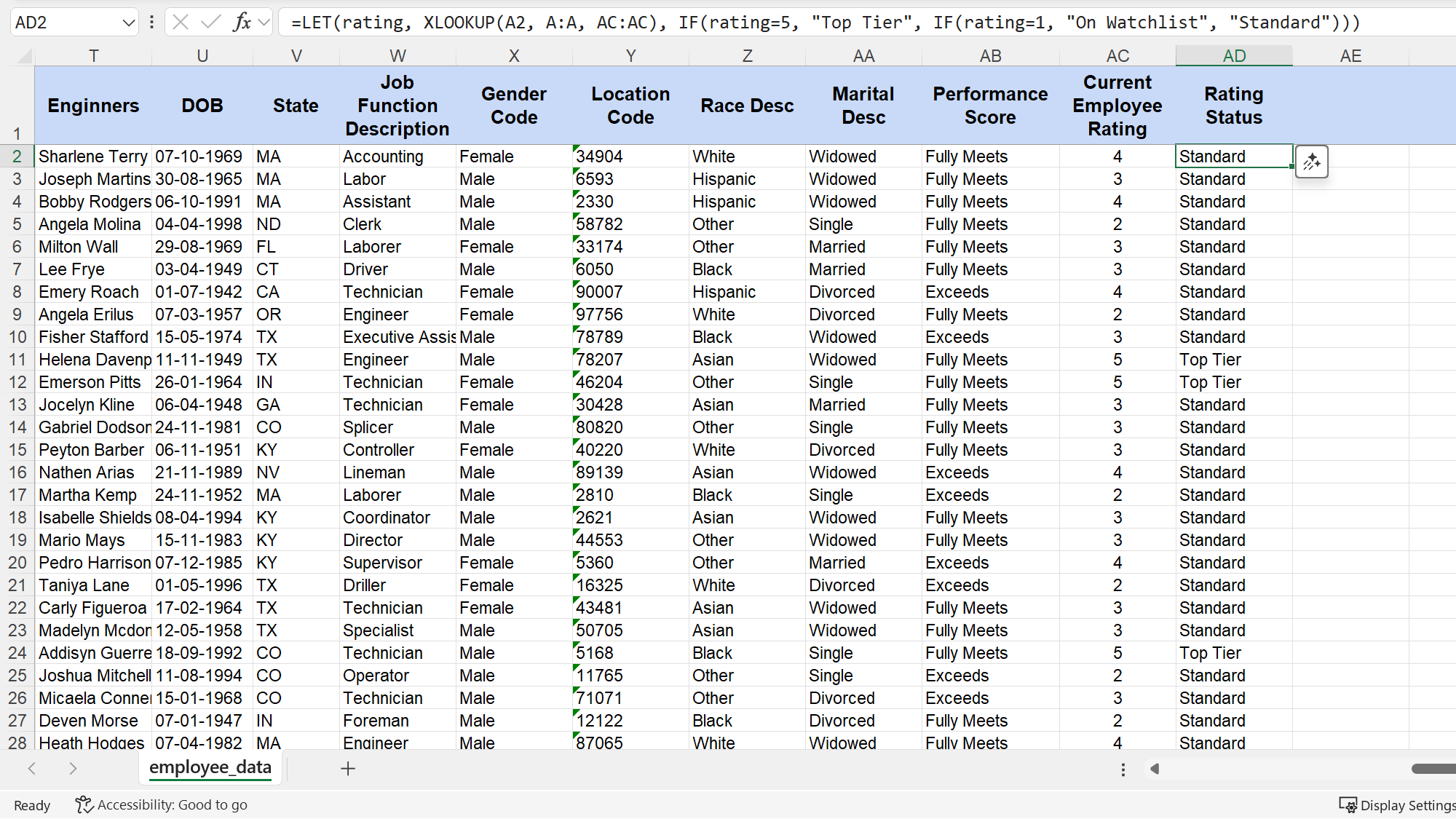
Let’s say I have a task that requires assigning a status based on an employee’s current rating. If their rating (found using their employee ID) is five, they are “Top Tier.” If it’s one, they are “On Watchlist.” Otherwise, they are “Standard.”
Without LET, I would have to write the XLOOKUP function twice, like the following:
=IF(XLOOKUP(A2, A:A, AC:AC)=5, "Top Tier", IF(XLOOKUP(A2, A:A, AC:AC)=1, "On Watchlist", "Standard"))
But with using LET, the formula becomes much cleaner. I calculate the XLOOKUP just once and assign it to the name “rating.”
=LET(rating, XLOOKUP(A2, A:A, AC:AC), IF(rating=5, "Top Tier", IF(rating=1, "On Watchlist", "Standard")))
This formula looks up an employee ID from cell A2 in column A, retrieves their numerical rating from column AC, and then categorizes the performance.
The LET function stores the rating lookup once, preventing Excel from repeating the same XLOOKUP calculation in the nested IF statements. The formula is significantly easier to read and debug.
2
INDEX and MATCH Work Great Together
They Create the Fastest Lookup Combinations
Before XLOOKUP existed, INDEX and MATCH were the only options for building fast lookups. Even now, this combination often outperforms newer functions in raw speed. On spreadsheets with tens of thousands of rows, this combination is noticeably faster because it processes only the specific columns you reference, not entire tables.
Neither function performs a complete lookup on its own. The MATCH function is good at one thing: finding the relative position (the row number) of a value within a column. Then, the INDEX function takes that number and fetches the corresponding value from another column.
First, let’s look at the MATCH syntax. It tells you where your data is.
=MATCH(lookup_value, lookup_array, [match_type])
- lookup_value: The value you want to find.
- lookup_array: The single column or row to search within.
- [match_type]: Use 0 for an exact match, which is what you’ll need 99% of the time.
Next is the INDEX syntax, which retrieves what you want based on the position MATCH provides.
=INDEX(array, row_num, [column_num])
- array: The range of cells or an array from which to retrieve a value.
- row_num: The row number from which to retrieve a value.
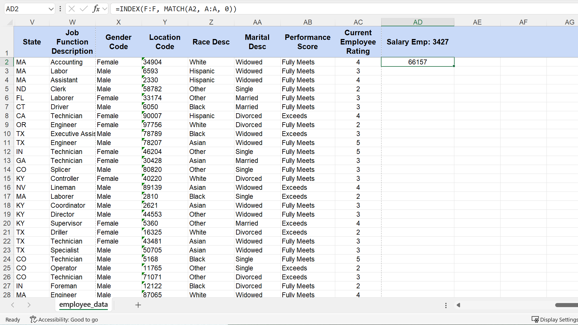
Let’s say I need to find the pay zone for the employee with ID 3,427. I would use the following formula:
=INDEX(F:F, MATCH(A2, A:A, 0))
In this example, the MATCH part first finds the row number for the employee ID located in cell A2. The INDEX part then takes that number and returns the value from that exact row in the pay zone column (which is column F). It’s a lightweight and efficient method.
1
FILTER Is the Ultimate Lookup Function
It Replaces Multiple Lookups at Once
Standard lookups, even XLOOKUP, have a fundamental limitation—they stop and return the very first match they find. But what if you need a list of all matching records? In Excel versions before 2021, this required complex array formulas. Now, I use the FILTER function instead. It extracts every single record meeting your criteria.
If you’ve never used Excel’s FILTER function, you’re seriously missing out. It dynamically returns an array of values that spills into the cells below the formula. This means you no longer need to guess how many results you’ll get. The function handles the output size for you, which is obviously a time-saver.
The following is the syntax of the FILTER function:
=FILTER(array, include, [if_empty])
- array: It is the entire range of data you want results from. This can be one column or many.
- include: This is your logical test. It’s a range of cells followed by a condition, like checking if a value in a column equals “Active”.
- [if_empty]: An optional argument for what to display if no results are found.
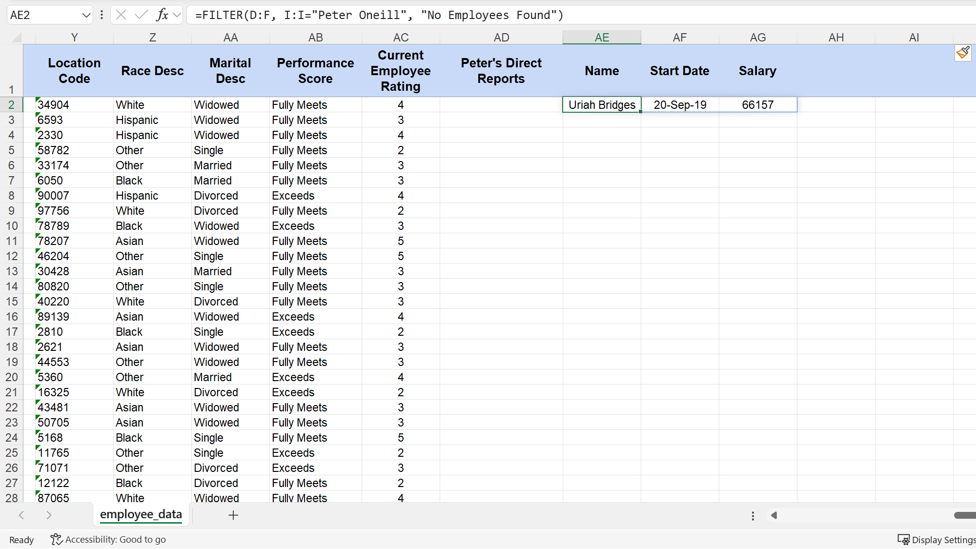
Let’s say a manager, Peter O’Neill, wants a list of all his direct reports. I need to pull the full name, start date, and salary for every employee who lists them as their supervisor. With FILTER, I can pull this entire list with just one formula instead of performing multiple individual lookups.
Here’s the formula that gets the job done:
=FILTER(D:F, I:I="Peter Oneill", "No Employees Found")
This formula tells Excel to return the data from columns D through F for every row where the value in column I is “Peter O’Neill.”
The results automatically populate the cells below, creating a clean, dynamic table. Because of this dynamic behavior, this Excel trick ends the pain of resizing tables forever.
These four approaches cover every lookup scenario I encounter. XLOOKUP is the modern replacement for VLOOKUP. I use LET combinations for optimization, INDEX/MATCH for pure speed, and FILTER for multiple results.
