Python’s SymPy Library Makes Math Easy. Here Are 6 Practical Uses

If the mention of algebra conjures bad memories of math classes, a Python library called SymPy could change your mind about the subject. With SymPy, algebraic operations become easier than tedious hand calculations and a lot more fun. Here’s what you can do with SymPy.

What Is SymPy?

SymPy is a computer algebra system, or CAS, library for Python. Where a numerical calculator operates on numbers, SymPy operates on symbolic expressions. It’s similar to Wolfram Alpha, Mathematica, and Maple, but completely free and open-source.

Other computer algebra systems use their own language, but since SymPy uses Python, if you know Python, you largely already know SymPy, apart from the specific library functions.

With SymPy, you can perform algebraic computations easily, solving equations, even calculus operations like differentiation and integration, without all those tedious hand calculations.

Before I get any math teachers on my case, if you’re in a class where you do have to show your handwritten work, SymPy is still a valuable educational tool. You can check your answers with SymPy, and you can explore concepts more easily than you can by hand. Working with mathematical software interactively encourages an exploratory mindset, where you can run “what if?” scenarios, such as changing the values of a function to see how the graph of it changes.

Installing SymPy

To install SymPy, you can use pip at the command line:

        pip install sympy
    

You can also use a tool like Conda, or Mamba, if you happen to use them.

On Mamba, to install into the current environment,

        mamba install sympy
    

Defining Variables

Before you can work with variables, you’ll have to define them with SymPy. The best way to work with SymPy is in an interactive session, such as in IPython or a Jupyter notebook.

To import all of Sympy into a session, use this command:

        from sympy import *
    

You’ll also want to enable “pretty-printing.” This will make SymPy’s output look more like what you’d see in a math or science textbook. In a Jupyter Notebook, Sympy will render the answer in LaTeX, a typesetting language widely used in STEM publishing.

Just use the init_printing method:

        init_printing()
    

With SymPy loaded in, we can start exploring its capabilities.

You can just type a number, such as 2, at the prompt:

        2

    

SymPy will print out a 2, rendered nicely. The main difference between the numerical operations you might be used to on a scientific calculator and a computer algebra system like SymPy will be that you’re dealing with floating-point approximations while SymPy deals with exact numbers and symbols.

Taking the square root with a numerical library versus in SymPy will clearly demonstrate this difference.

Let’s take the square root with NumPy first:

        import numpy as np
np.sqrt(2)
    

You’ll get a numerical approximation, since 2 is not a perfect square.

Compare this with SymPy’s result:

        sqrt(2)

    

Since this isn’t a perfect square, SymPy will just leave it unevaluated. You can get a numerical approximation if you want one with the N function.

        N(sqrt(2))
    

Alternatively, you can append a .evalf() to an exact operation you want a numerical approximation of.

        sqrt(2).evalf()
    

I prefer the former because “N” for “numeric” seems easier to remember to me. It’s also similar to how other mathematical programs like Mathematica work.

More interesting is the way SymPy handles square roots that do contain perfect squares:

        sqrt(56)
    

SymPy will automatically factor out perfect squares from square roots.

To perform algebraic operations, you have to declare symbolic variables. Let’s take some inspiration from René Descartes and define the classic x and y variables with the symbols function:

        x,y = symbols('x y')
    

Notice that between the variables in the symbols function, you don’t type a comma, but a space instead.

If we just type them at the prompt, they’ll be printed by themselves.

        x
y
sqrt(x)
    

Basic Algebraic Operations

With the variables defined, we can perform operations with them. If you take the square root of x, it will display the unevaluated square root under the radical symbol, just as we did with 2 earlier

        sqrt(x)
    

We can also define other operations, such as adding, multiplying, and dividing variables

        x*2
x*y
2*x * y
2*x + 3*y
x / y
(2*x) / y
    

When writing out algebraic expressions by hand, you can ignore the multiplication sign, you’ll need to make the multiplication explicit using Python’s * operator.

The parentheses are there to group the 2x operation, so SymPy won’t think we’re trying to divide x by y and then multiply that by 2.

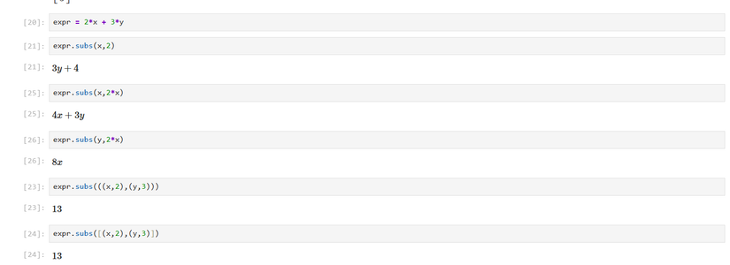
You can also substitute variables in algebraic expressions with Sympy.

Let’s define an expression:

        expr = 2*x + 3*y
    

We can use the subs method of an expression to substitute a variable for a value by supplying the variable and the value you want to substitute it for:

For example, to substitute 2 for x:

        expr.subs(x,2)

    

You can also substitute other expressions:

        expr.subs(x,2*x)
    

Expansion and Factoring

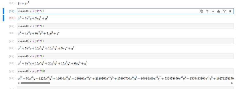
While you can perform basic arithmetic operations in SymPy, it won’t multiply polynomials by each other unless you tell it to.

A binomial expression like this will remain unevaluated:

(2*x + 3*y) * (5*x**2 - 4*y)

To get the results of these polynomials multiplied, use the expand function:

        expand((2*x + 3*y) * (5*x**2 - 4*y))
    

This will multiply these two polynomials together using the distributive property.

The same thing works for bigger expressions, such as a binomial multiplied by a trinomial:

        expand((2*x + 3*y) * (5*x**2 - 4*y))
    

You can also factor expressions to do the opposite, to return an expanded operation to its original form:

        factor(10*x**3 + 15*x**2*y - 8*x*y - 12*y**2)
    

Solve Equations

You could spend all day expanding and factoring expressions, but what SymPy is really useful for is solving equations.

The simplest equations to solve are linear equations, such as 5*x – 3 = 0

You can solve any equation that equals 0 with the solve function:

        solve(5*x - 3,x)
    

The expression is the first argument, followed by the variable you want to solve for.

If you have an equation like 2x + 3 = 30, you can either rearrange the equation so that it’s equal to 0 or use an Eq object. For the first method, you’d subtract 30 from both sides and solve for x:

solve(2*x + 3 - 30,x)

An equality object will let you represent equations in a more familiar form. You call the Eq function and supply a tuple with both sides of the equation.

eq = Eq(2*x + 3,30)

You can solve it using the solve function as before.

        solve(eq,x)
    

Either way, you’ll get the results in a list. To get access to the values, such as to use them in another function, you can save them in an array:

        solutions = solve(eq,x)
    

While simple linear equations are trivial to solve by hand, quadratic equations are harder. They’re also easy to solve with Sympy:

        solve(x**2 + 2*x + 3,x)
    

You can even solve systems of equations:

        eqn1 = Eq(3*x + 4*y,15)
eqn2 = Eq(5*x - 3*y,30)
solve([eqn1,eqn2],[x,y])
    

The square brackets indicate that these are lists. You can also use matrices to solve systems of linear equations in a more compact way, which I’ll demonstrate later.

Making Plots

SymPy lets you replace your graphing calculator by making plots of functions. You can use the built-in plot function. Let’s plot a simple linear equation:

plot(2*x + 3)

The format for linear equations should be in the familiar slope-intercept form, y = mx + b, where “m” is the slope. By default, the plot function will plot the x values or any value in an equation from -10 to 10. This also applies to any variable you put in there.

You can change this by supplying a tuple of the variable, the lower bound, and the upper bound. To see the plot between x between 2 and 5:

        plot(2*x + 3,(x,2,5))
    

The same applies to polynomials, such as the quadratic we solved earlier:

        plot(x**2 + 2*x + 3)
    

Calculus and Linear Algebra

While they can easily tackle elementary algebra, computer algebra systems like Mathematica and Maple are widespread in the sciences because they make calculus and linear algebra, both of which are ubiquitous in STEM but tedious to perform by hand, more manageable. These calculations even pop up in social sciences such as economics.

I’m not going to explain the theory very much, but if you’re interested in learning more about calculus and linear algebra, there are a lot of off-and-online resources available, such as Khan Academy and OpenStax’s free textbook. Their college algebra textbook also describes solving linear systems of equations with matrices. Khan Academy also has a series on linear algebra.

To take a derivative with respect to a variable, use the diff function:

diff(x**2 + 2*x + 3,x)

Integrals work the same way with the integrate function:

integrate(x**2 + 2*x + 3,x)

The output does not include the constant of integration, though.

You can compute the definite integral over an interval with a method similar to the plotting function shown earlier. For example, to calculate the area under the curve for the previous function for values of x between 0 and 2:

        
integrate(x**2 + 2*x + 3,(x,0,2))

    

Solving systems of linear equations is also easy with SymPy. We can create a random 3×3 square matrix with the randMatrix function and then look at it:

        A = randMatrix(3)
A
    

We can create our column vector of variables we want to solve for in a similar way, creating a single column with three rows, or a 3×1 matrix:

        b = randMatrix(3,1)
    

Let’s take the determinant so we can be sure this system has a unique solution:

        det(A)
    

Since the determinant is nonzero, we can proceed with solving this system. The coefficient matrix we created has a solve method that we can use with the column vector as the argument:

        A.solve(b)

    

In practice, using NumPy for a numerical solution might be faster.

---

With SymPy, you can take the pain out of symbolic math by turning Python into a super calculator. If you never thought of yourself as a “math person,” using SymPy could turn you into one.