Picture this: you’ve created an all-singing-all-dancing Microsoft Excel workbook, but when you share it with others, they have no idea where to start. That’s why you need a homepage worksheet that provides all the important information and links as soon as people open the file.
By the end of this guide, you’ll have a homepage worksheet looking something like this.

Set Up Your Homepage Worksheet
Before you start adding content to your homepage worksheet, take a few moments to get everything set up and formatted. Taking this step now is sure to save you time down the line.
First, reduce all the column widths so you’re not bound to the default setting. In other words, by doing this, you’re giving yourself more freedom in terms of where you can start a line of text or add a graphic. To do this, click the “Select All” button in the top-left corner of the worksheet, and click and drag one column to make it smaller.

Next, reduce the width of column A even further, so that you have a small margin separating the edge of the workbook and the content you’ll add soon.

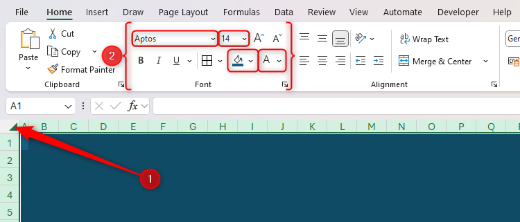
Now, it’s time to decide what color you want the background, which font you want to use, and how big the text will be.
Again, click the “Select All” button in the top-left corner, and in the Home tab on the ribbon, choose a cell fill color, a font, a text size, and a font color. In my case, I’ve chosen a dark teal background, used the default font (Aptos) in white, and chosen 14pt as the standard text size.
Related
Which Fonts Should You Use in Excel?
Optimize your data’s readability.
Now that you’ve set up your worksheet, it’s time to start adding content.
Welcome Your Collaborator
Your homepage worksheet should be similar to a homepage on a website—it should be welcoming, and viewers should be able to instantly see what’s going on. That’s why the first two elements you need to add are a title and an intro line.
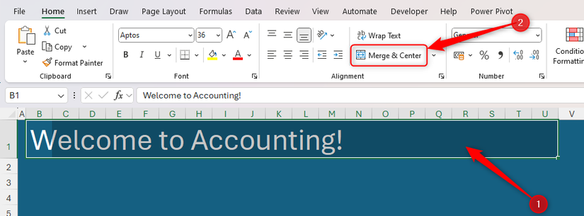
Providing you’ve created a margin column, in cell B1, type your welcoming title, press Enter, and format the text so that it stands out.

Then, decide how wide your homepage worksheet is going to be, making sure that all the content will be visible to people using different monitor sizes. To do this, select all the cells from B1 to the last column that will form the homepage worksheet, and click “Merge And Center” in the Home tab on the ribbon.
Now, in cell B2, add a brief intro line that explains what the workbook contains, and merge and center the cells as you did in row 1.

Add Hyperlinks to Key Worksheets
Even though collaborators can click the worksheet tabs at the bottom of the Excel window to jump between the different sheets, adding a banner of links beneath the title and intro makes the homepage worksheet even more user-friendly.
You’ll need to already have created the other worksheets in your workbook before you can link to them. To add a worksheet, click the “+” next to the worksheet tabs at the bottom of the Excel window, and double-click a tab to rename it.
In my case, aside from the homepage worksheet, my workbook has five worksheets, so I’ll create five tab-like links. Since there are 20 columns from column B to column U, each of my links needs to be four cells wide.

Related
3 Ways to Insert Hyperlinks in Microsoft Excel
It just makes things easier when you can click a link.
So, I’ll color cells B4 to E4 yellow, F4 to I4 light orange, J4 to M4 light green, N4 to Q4 light purple, and R4 to U4 red by selecting the cells, and clicking the “Fill Color” drop-down option in the Home tab. At the same time, I’ll merge and center each set of four cells to turn them into larger whole cells.

Now, populate each colored tab in this menu bar with the names of the other worksheet tabs to which they’ll be linked. You might need to change the font colors so you can see what you’ve typed, but don’t worry about applying final formatting to the text just yet—we’ll do this shortly.

The next step is to link each of these colored tabs to the individual worksheets. To do this, right-click the first tab, and select “Link.” Alternatively, select the cell, and press Ctrl+K.

Now, in the Insert Hyperlink dialog box, click “Place In This Document,” select the relevant worksheet, and click “OK.”

Repeat this process for all the links in the homepage banner until all the text is blue and underlined.

The default link formatting (blue and underlined) can make the text difficult to read. So, select all the cells in the banner, increase their font size, and make sure the font colors don’t clash with the background. I also like to remove the underlined formatting to make things look a little tidier.

Finally, click the links to make sure they take you to the right worksheet.
Display the Next Key Date
Your primary aim when designing a homepage worksheet is to prioritize the important info and structure the page accordingly. That’s why, in a corporate setting, the next thing to add is a critical message that everyone will see. In my example, I’m going to display the details of the next deadline.
As you can see, I’ve added a sub-heading, increased its font size, merged and centered the row so that it covers the whole width of the homepage worksheet, and added a white border to the bottom of the merged cell.

Now, before I add the details, I’m going to add an appropriate icon via the Insert tab on the ribbon. This helps break up the homepage worksheet, works well for people who prefer visual content, and helps me reduce the proportion of text on the sheet.
If you wish to do the same, first, in the Insert tab on the ribbon, click “Icons.” Then, in the search field of the Stock Images dialog box, type a keyword linked to the icon you want to add, and once you’ve found and selected one that’s ideal, click “Insert.”
Now, reposition and resize the icon, and change its color in the Graphics Format tab on the ribbon. Then, start adding the relevant text where you will display the deadline details.

Although you could add this information manually, making it update automatically is much more efficient. First, on a separate worksheet, list all the deadline dates in chronological order in column A, and state the details of each deadline in the corresponding cells in column B.

Then, on the homepage worksheet, select the cell where you want the next deadline date to be inserted, and make sure it’s formatted as a short date in the Number group of the Home tab on the ribbon.


Related
Excel’s 12 Number Format Options and How They Affect Your Data
Adjust your cells’ number formats to match their data type.
Now, type:
=MIN(FILTER(Deadlines!A:A,Deadlines!A:A>TODAY()))
where Deadlines! is the reference to the sheet where the deadlines are listed, and A:A references the column containing the dates.
When you press Enter, the next deadline in this list will be inserted into your homepage worksheet. In my example, I’ve merged and centered cells G8 to J8 so that the date fits nicely into its allotted cell.

Now, use a simple XLOOKUP formula in the cell where you want the task details to be displayed:
=XLOOKUP(G8,Deadlines!A:A,Deadlines!B:B)
where G8 is the cell containing the date, Deadlines!A:A looks up that date in column A of the Deadlines spreadsheet, and Deadlines!B:B returns the corresponding details.

Impressively, once a deadline passes, Excel will automatically look for the next deadline date and update the information accordingly.
Tell People How the Workbook Works
Now that you’ve got the important stuff out of the way, it’s time to help people understand how to navigate and read the file. After all, having a super-complex workbook is no good if people can’t use it properly!

This section of your homepage worksheet is essentially a key to the nuts and bolts of your workbook. It explains what people might encounter when they jump between the worksheets and what they should do in those situations.

Related
6 Ways to Make Your Excel Spreadsheet Easy to Read
Six tried and tested ways to show off your spreadsheet.
In this example, as well as emphasizing that the collaborator can use the banner at the top of the page to navigate the workbook, I’ve made it clear that light blue cells are open for data entry, my coworkers can hover over any cell with a red marker to see more information, and they can also click the Home button at any time to return to the welcome page.

Notice how I’ve added icons (via the Insert tab on the ribbon) to some of the instructions to add visual quality to the homepage worksheet, as well as examples to make things clearer. That said, regardless of how you design this section, the key is to not have too many instructions—keeping the how-to part short and sweet is the best way to increase the chances of people reading it.
Let Coworkers Know Where They Can Get Help
Even though you’ve added a section that guides people through your workbook, there’ll inevitably be questions that remain unanswered. That’s why you should include a section in your homepage worksheet that directs people to support.
Here, the icons (added through the Insert tab on the ribbon) and text are hyperlinked to different places:
- See FAQs: This text and the question mark icon are linked to another worksheet in the workbook where frequently asked questions and their answers are displayed.
- Visit intranet: This text and the web icon are linked to the URL of a local network page that contains essential information.
- Email Tom: People who click this text or the corresponding icon will be taken to their default email program, and a blank email to Tom will be generated with the subject Help with Accounting workbook.

You can add these different types of links by selecting the cell or icon, pressing Ctrl+K (or right-clicking and selecting “Link”), and choosing one of the three options in the left-hand pane of the Insert Hyperlink dialog box.

Remember that you’ll need to reformat any text to which you add hyperlinks, since Excel automatically turns hyperlinks blue.
Include a Data Snapshot
The final section of the Excel homepage worksheet should contain a snapshot of important figures, keeping people up-to-date with the key metrics of your organization each time they open the workbook.

Related
Your Excel Spreadsheet Needs a Dashboard: Here’s How to Create One
Have your KPIs in one place.
One way to do this is to create new charts for existing data in your workbook by selecting the data, and choosing from a chart type in the Insert tab on the ribbon.

You can then cut and paste the chart onto your homepage worksheet.
If you’ve already created charts in other worksheets and want to duplicate them on your homepage worksheet, you can use the Camera tool. This useful feature lets you take a shot of your chart and paste it as an image. However, unlike normal images, those you create using the Camera tool are dynamic, meaning they update to reflect any changes in the original data.
First, since the Camera tool isn’t visible by default, you need to add it to your Quick Access Toolbar (QAT). To do this, click the QAT down arrow, and select “More Commands.”

If you can’t see the QAT, right-click any tab on the ribbon, and select “Show Quick Access Toolbar.”
Next, select “All Commands” in the Choose Command From menu, and scroll to and select “Camera.” Next, click “Add” to add it to your QAT, and finally, click “OK.”

Now, you can see the Camera icon added to your QAT.
To capture a chart with this tool, select all the cells behind and surrounding the chart, and click the “Camera” icon in your QAT.

Then, head back to your homepage worksheet, and click anywhere to paste the copied data. Since Excel treats this as an image, you can use the handles to resize the graphic, as well as the Picture Format tab on the ribbon to present the snapshot exactly as you want, including cropping the edges.

Now, repeat this process for any other graphics or charts you want to include as data snapshots on your homepage worksheet.

Hide the Column and Row Headings
Now that you have added all the necessary content to your homepage worksheet, you can make one final tweak to improve its appearance.
There’s no need for the column and row headings (A, B, C, and so on at the top of the spreadsheet, and 1, 2, 3, and so on down the left) to be on display in this worksheet. In fact, they take up valuable real estate and could cause confusion.
So, to hide them, in the View tab on the ribbon, uncheck “Headings.”

This new setting only applies to the active worksheet and remains intact when you share the workbook with others.
In truth, your homepage worksheet can contain anything you think will help people with whom you share the workbook. As long as you provide only the necessary tidbits of info, include subtle graphics to divert people’s eyes to the important bits, and create the impression that the workbook is easy to use, your homepage worksheet will serve its purpose.