Excel is powerful, but its formulas can get unwieldy fast. I found a way to simplify even the most bloated ones without losing functionality, and it’s been a total game-changer for my spreadsheets.
What Is the LET Function?
LET is a function in Excel that allows you to add variables to your formulas to make them more manageable and efficient.
Think of variables like containers with labels that store different values, such as numbers or text. They make the values easier to reuse and manipulate, especially if they’re the result of intermediate calculations. That’s because you can refer to them using the name of their respective container instead of directly.
Here is the syntax of the LET function:
=LET(variable_name_1, value_to_assign_1, [variable_name2, assigned_value2, ...], final_calculation)
In the syntax, variable_name_1 is the name or label of the variable you want to use. For instance, if it’s going to store the weight of something, you can simply call it weight. The value_to_assign_1 parameter is the value you want to assign to variable_name_1.
You can also create more variables and assign names to them, which is where the optional [variable_name2, assigned_value2, …] argument comes in. And final_calculation is the formula that uses the named variables to produce a result.
LET is one of those Excel functions that can save you tons of work in the long run. However, it requires everyone looking at the Excel sheet to grasp the concept of variables, on top of how the function works. It’s worth learning, though, as we will see with the example in the next section.
How the LET Function Makes Formulas More Readable
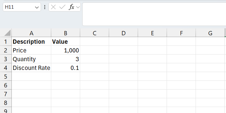
The best use case of the LET function is to reduce the complexity of formulas with several intermediate calculations. Let’s look at the sample data below that shows the price, quantity, and discount rate of an item.
We are going to use basic math in Excel to figure out the total cost of the product after factoring in everything. Here’s the syntax of the calculation:
total_cost = subtotal - (subtotal * discount_rate)
Let’s break down what is happening here:
- First, we need to calculate subtotal, which is the price (A2) multiplied by the quantity (A3).
- Second, we need to know the discount amount, which is subtotal multiplied by the discount rate (A4).
- Finally, we get the total cost by subtracting the discount amount from the subtotal.
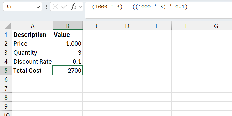
Here is what the formula would look like in Excel if we hard-coded the values:
=(1000 * 3) - ((1000 * 3) * 0.1)
There are a couple of problems here that make this formula complex. The most glaring one is that the calculation for the subtotal (1000 * 3) is repeated twice, making the formula hard to read. It’s also bad for performance, since Excel is repeating the calculation instead of just reusing the result.
Also, imagine if we had repeated it several more times in the formula. That means if we changed something in that calculation, we’d also have to change it everywhere it’s repeated. That’s a tedious and error-prone process.
Also, it’s hard to tell what the numbers mean by themselves. For instance, when calculating subtotal, is the 1000 the quantity or the price of the item? There is nothing that makes it obvious what those numbers are.
It also doesn’t become much easier to read if we use cell references, like in the example below:
=(B2 * B3) - ((B2 * B3) * 4)
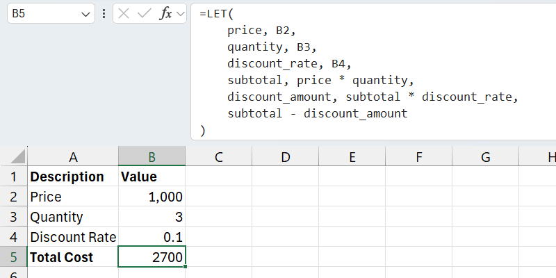
When we use the LET function, the formula becomes more readable because we build it up slowly, removing the complexity with each step. Here is what it would look like (I will put everything in a separate line to make it easier to follow the example):
        =LET(
    price, B2,
    quantity, B3,
    discount_rate, 4,
    subtotal, price * quantity,
    discount_amount, subtotal * discount_rate,
    subtotal - discount_amount
)
Here, the values in A2, A3, and A4 become more descriptive with price, quantity, and discount_rate, respectively. Now we just use those named variables to calculate subtotal and discount_amount. As you can see, every value is assigned to a variable once, either by referencing a cell or storing the result of an intermediary calculation, and then reused throughout.
Furthermore, it’s easier for someone else to trace how you calculated the total cost. And if we change the values in the variables (e.g., use another cell reference or add another variable to the intermediary calculations), we don’t have to go around tweaking the formula in multiple places.
Rules to Keep in Mind When Naming Variables
Before you go about using the LET function with your formulas, it helps to learn some rules and best practices when naming your variables.
Keep the following in mind:
- Ensure the names are descriptive of the value you’re going to assign to them.
- Names can contain letters and numbers.
- Don’t use names reserved by Excel (e.g., SUM, MAX, or IF).
- You cannot use spaces when naming variables, so if you want to separate words, use CamelCase (e.g., discountAmount) or snake case (e.g., discount_amount).
- Use the same naming conventions consistently throughout—avoid combining CamelCase and snake case.
- Don’t use special characters other than the underscore.
Functions like LET make your formulas human-readable, which is great for collaboration. On top of that, if you come back and look at your formulas months down the line, it’s much easier to remember what they do if you have descriptive names. It’s a very useful function that significantly cuts complexity by simplifying how you interact with formulas, even if they end up being more verbose.


