When you think of double quotation marks, you probably remember your English lessons in school. However, in Microsoft Excel, they serve a different purpose altogether. In fact, they can help you improve your formulas, let you interact with AI, and make your spreadsheets tidier.
Including Text Strings in Formulas
One of the most common uses of double quotes in Microsoft Excel concerns text strings in formulas.
Imagine you’re a teacher. In your Excel worksheet, you have this table, with student IDs in column A, their scores in column B, and a blank Status column where you will evaluate their scores.
Specifically, if a value in the Score column is 50 or more, you want to return the word Pass in the corresponding row of the Status column. On the other hand, if a value in the Score column is less than 50, you want to return the word Fail.
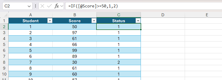
Before I show you the formula for this, let’s go back a step and imagine that, rather than returning the words Pass or Fail, you wanted to return the numbers 1 or 2. For this, the IF formula would be as follows:
=IF([@Score]>=50,1,2)
meaning if a score in a given row is greater than or equal to 50, the result is 1. If it’s not, the result is 2.
When you enter a formula into a cell in a column of an Excel table and press Enter, it is automatically duplicated in the remaining cells of the same column. This saves you from having to use the fill handle or copy and paste the formula manually.
Because the return values in the formula are numbers, you don’t need to use any double quotes. However, turning back to the return values Pass and Fail, because these are text, you do need to use double quotes:
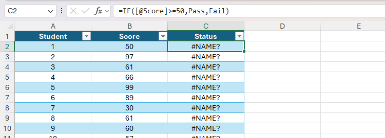
=IF([@Score]>=50,"Pass","Fail")
If you don’t embed these values in double quotes, you’ll see the #NAME? error because Excel is looking for numerical return values, but can’t find any.
In the example above, you saw that double quotes are used to define textual results in a logical formula. However, the same principle applies to any arguments containing text in any formula.
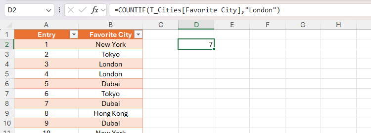
Here, the formula in D2, which uses the COUNTIF function to count the number of times the word London appears in the Favorite City column of the T_Cities table, uses quotation marks around the lookup value:
=COUNTIF(T_Cities[Favorite City],"London")
Failing to include the quotation marks in this case would return zero because Excel can’t link the lookup value to the specified range.
An arguably better way to achieve the same outcome as in the example above is to type the word London into a separate cell, and reference that cell in the lookup value argument instead. Using cell references instead of hard-coding values in formulas has many benefits—one is that you don’t need to remember to use double quotes when referencing cells.
Defining Prompts When Using the COPILOT Function
Excel’s COPILOT function uses artificial intelligence to generate responses according to a prompt you input.
At the time of writing (August 2025), the COPILOT function is in preview with Microsoft Insiders. Microsoft warns that the COPILOT function “uses AI and can give incorrect responses,” advising that you should use “native Excel [functions] for any task requiring accuracy or reproducibility.”
Here’s the syntax:
=COPILOT(prompt¹, [context¹], [prompt²], [context²], ...)
where each prompt is the text that describes the task or question, and each context directs Excel to the relevant single cell, range of cells, table, or named range.
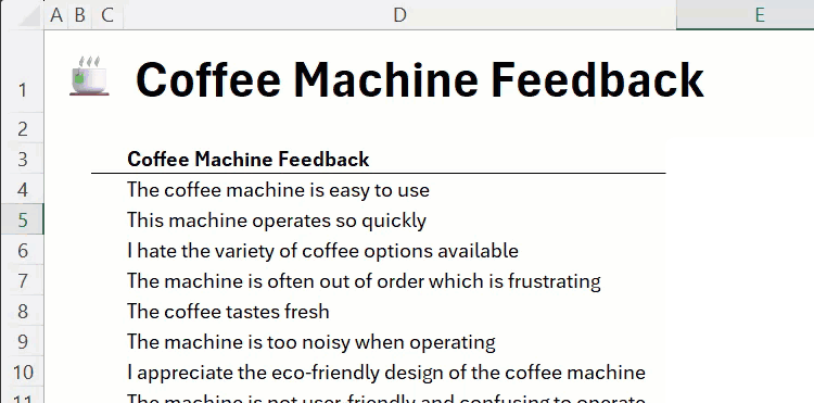
Suppose you’ve gathered some feedback from your coworkers on a new coffee machine you installed in the office.
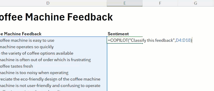
Now, you want to use the COPILOT function to classify the comments into positive and negative. To do this, in cell E4, make sure the prompt argument is embedded within double quotes:
=COPILOT("Classify this feedback",D4:D18)
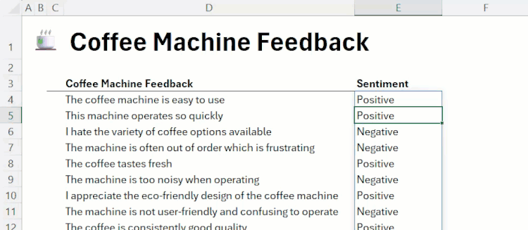
Here’s what you’ll see when you press Enter:
Because the context argument is a range of cells, the result is a dynamic array, meaning it spills over from the cell where you typed the formula.
If you forget to put quotes around a prompt in the COPILOT formula, Excel returns a #VALUE error.
Representing and Returning Blank Cells (Empty Strings)
One of the most practical uses of double quotes in Excel is to represent—well—nothing! Absurd as this might sound, it’s a great way to keep your spreadsheet tidy and free of formula error alerts.
In this example, let’s say you only want the total score for each player to show once they’ve completed all three rounds. If they haven’t completed all three rounds, you want the corresponding cell in the Total column to be blank.
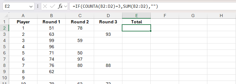
To do this, in cell E2, type:
=IF(COUNTA(B2:D2)=3,SUM(B2:D2),"")
and press Enter.
I’ve used a regular range (as opposed to an Excel table) in this example so that the formula is shorter and easier to read.
As you can see in the screenshot above, cell E2 is blank, even though it contains a formula including a SUM argument. Here’s why:
If there are three non-blank cells in the range B2 to D2 (IF(COUNTA(B2:D2)=3), their values are added together (SUM(B2:D2)). However, if the number of non-blank cells in the range B2 to D2 does not equal three, the formula returns a blank cell, as determined by two double quotes placed one after the other (“”) as the final argument of the IF formula.
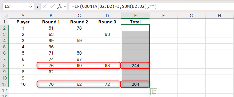
When I double-click the fill handle in the bottom-right corner of the selected cell E2 to apply the formula to the other cells in column E, only the totals where all the corresponding values in columns B, C, and D are returned.
So, the double quotes come in handy in this scenario because incomplete totals are hidden, meaning analyzing the completed totals is easier.
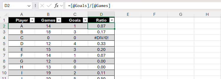
One of my favorite uses of double quotes in Excel is with the IFERROR function. In this example, I am tracking the goals-per-game ratio of ten players. To do this, I typed:
=[@Goals]/[@Games]
in cell D2, and when I pressed Enter, the Excel table automatically duplicated the formula down the rest of the column.
However, because player C has not played any games, the formula returns #DIV/0! in cell D4.
To tidy this up, I can embed the whole formula within the IFERROR function:
=IFERROR(x,y)
where x is the calculation being performed, and y is the value to return if there is an error.
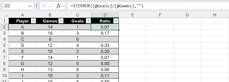
In this case, the calculation is to divide the values in the Games column by the values in the Goals column, and the if-error value should be a blank cell, represented by two double quotes:
=IFERROR([@Goals]/[@Games],"")
As a result, the error is hidden.
Because the formula still contains the division calculation, as soon as I enter a value greater than zero in cell B4, the division can be performed, so a value is shown.
Bear in mind that using the IFERROR function to hide errors in your spreadsheet can make identifying calculation errors more difficult. This is why I only tend to use it in scenarios when #DIV/0! would otherwise appear.
Adding a Space (Delimiter) When Joining Text
There are many ways to join text in Microsoft Excel, including using the ampersand (&) symbol or a selection of functions. However, if you want to add a delimiter between two values you merge, this is where double quotes come into play.
A delimiter is a character, symbol, or space used to separate items in a sequence. So, for example, the delimiter between a first name and a last name is a space, and the delimiter between a file’s name and extension is a period.
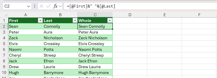
Let’s say you want to take these people’s first names (column A) and last names (column B), and join them together in column C. However, importantly, you need to leave a space between each of the two names.
One way to do this is by using the ampersand:
=[@First]&" "&[@Last]
where
- [@First] takes the name from the column named First,
- ” “ (double quotes either side of a space) tells Excel to add a space delimiter,
- [@Last] takes the name from the column named Last, and
- The ampersands link all of the above to produce a string.
Another way to merge the first and last names with a space between is by using the TEXTJOIN function:
=TEXTJOIN(" ",TRUE,[@First],[@Last])
where
- ” “ (a space between two double quotes) tells Excel that the delimiter between each joined text value is a space,
- TRUE tells Excel to ignore blank values (whereas FALSE would include blank values),
- [@First] takes the name from the column named First, and
- [@Last] takes the name from the column named Last.
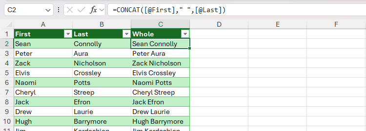
You can also use the CONCAT function to achieve the same outcome:
=CONCAT([@First]," ",[@Last])
where the CONCAT function joins each argument together—one of which is a space, which separates the text extracted from the First column from the text extracted from the Last column.
In all the examples above, you could insert a character—such as a period, hyphen, forward slash, or asterisk—between the double quotes, instead of a space.
Displaying Quotation Marks in Text Strings
You might be wondering how to actually display double quotes in text. This is where things can get complicated. But don’t worry—there’s an easier way to get around it.
Suppose you want to display the following in an Excel cell: She said, “Hello.”
Typing:
=She said, "Hello"
into a cell and pressing Enter would cause Excel all sorts of confusion and return an error, because the formula contains text that isn’t wrapped in double quotes.
OK, so let’s wrap the whole thing in double quotes:
="She said, "Hello.""
This doesn’t work either, because the first double quote starts the text string, and Excel thinks that the second double quote ends it. So, everything from the word Hello onward can’t be understood.
This time, let’s add some more double quotes around the word Hello:
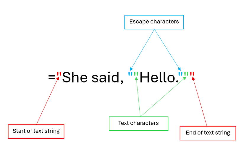
="She said, ""Hello."""
This time, you get the intended result.
This is because when two double quotes are used together, the first is an escape double quote, and the second is an actual double quote, treated as text. So, in the formula above, the first double quote signifies the start of the text string, the second is the escape character for the third, the fourth is an escape character for the fifth, and the sixth signifies the end of the text string.
If seeing so many double quotes hurts your head (as it does mine!), there’s an easier-to-understand approach. Typing:
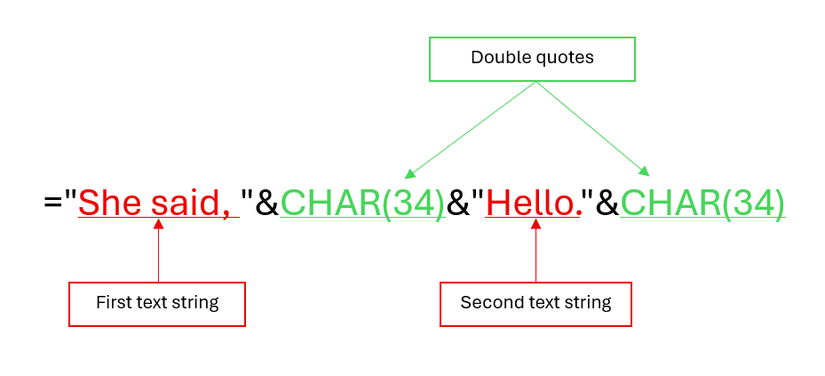
="She said, "&CHAR(34)&"Hello."&CHAR(34)
and pressing Enter returns the same intended result.
This is because the double quotes on either side of the text tell Excel you want to return a text string, and CHAR(34) is the code to return a double quote as text.
Double quotes aren’t the only special characters in Excel that serve a specific purpose. For example, even though parentheses, square brackets, and curly braces look similar, they all have very particular functions. And on the topic of symbols, it’s also worth getting to know what the hash (#) sign does in Excel.

